An Apache Airflow MVP: Complete Guide for a Basic Production Installation Using LocalExecutor

An Apache Airflow Pipeline. Souce: Unsplash### Recap

In the first post of our series, we learned a bit about Apache Airflow and how it can help us build not only Data Engineering & ETL pipelines, but also other types of relevant workflows within advanced analytics, such as MLOps workloads.

We skimmed briefly through some of its building blocks, namely Sensors, Operators, Hooks and Executors. These components provide the basic foundation for working with Apache Airflow. Back then, we worked with the SequentialExecutor, the simplest possible Airflow setup. Having support for running only one task at a time, it is used mainly for simple demonstrations. That is obviously not enough for production scenarios, where we might want to have many tasks and workflows being executed in parallel.

As we already discussed, Apache Airflow ships with support for multiple types of Executors — each of them is more suited to a particular type of scenario.

• LocalExecutor unleashes more possibilities by allowing multiple parallel tasks and/or DAGs. This is achieved by leveraging a full fledged RDBMS for the job metadata database, which can be built on top of a PostgreSql or MySQL database. While you can definitely run some light production workloads using LocalExecutor, for scaling up you would have to resort with vertical scaling by beefing up the hardware resources of your environment.
• CeleryExecutor addresses this limitation: it unlocks the possibility of scaling the setup horizontally by allowing you to create a processing cluster with multiple machines. Each machine spins up one or more Celery Workers in order to split Airflow’s workload. Communication between workers and the Scheduler is performed through a message broker interface (can be implemented using Redis or RabbitMQ). Having said that, you must define the number of workers beforehand and set it up in Airflow’s configuration, which can make the setup a bit static.
• DaskExecutor works in a similar way as CeleryExecutor, but instead of Celery, it leverages the Dask framework for achieving distributed computing capabilities.
• More recently, KubernetesExecutor has become available as an option to scale an Apache Airflow setup. It allows you to deploy Airflow to a Kubernetes cluster. The capability of spinning Kubernetes Pods up and down comes out of the box. You will want to use such setup if you would like to add more scale to your setup, in a more flexible and dynamic manner. However, that comes at the expense of managing a Kubernetes cluster.

An Apache Airflow MVP

When starting up a data team or capability, evaluating cost versus benefit as well as complexity versus added value is a critical, time consuming, daunting task. Agile organizations and startups usually work with prototypes to tackle such scenario — sometimes working products are better at answering questions than people.

Inspired by this philosophy, we will create a basic, hypothetical setup for an Apache Airflow production environment. We will have a walkthrough on how to deploy such an environment using the LocalExecutor, one of the possible Apache Airflow task mechanisms.

For a production prototype, choosing LocalExecutor is justified by the following reasons:

• Provides parallel processing capabilities
• Only one computing node — less maintenance & operations overhead
• No need for Message Brokers

LocalExecutor

You might be asking — how is that possible? Well, as the name indicates, when we use the LocalExecutor we are basically running all Airflow components from the same physical environment. When we look at the Apache Airflow architecture, this is what we are talking about:

Main Airflow Components for a LocalExecutor Setup. Source: AuthorWe have multiple OS processes running the Web Server, Scheduler and Workers. We can think of LocalExecutor in abstract terms as the layer that makes the interface between the Scheduler and the Workers. Its function is basically spinning up Workers in order to execute the tasks from Airflow DAGs, while monitoring its status and completion.

Getting The Wheels Turning

We had a conceptual introduction on LocalExecutor. Without further ado, let’s setup our environment. Our work will revolve around the following:

1. Postgresql Installation and Configuration
2. Apache Airflow Installation
3. Apache Airflow Configuration
4. Testing
5. Setting up Airflow to run as a Service

These steps were tested with Ubuntu 18.04 LTS, but they should work with any Debian based Linux distro. Here we assume that you already have Python 3.6+ configured. If that’s not the case, please refer to this post.

Note: you could also use a managed instance of PostgreSql, such as Azure Database for PostgreSql or Amazon RDS for PostgreSql, for instance. This is in fact recommended for a production setup, since that would remove maintenance and backup burden.

1. Postgresql Installation and Configuration

To install PostgreSql we can simply run the following in our prompt:

sudo apt-get install postgresql postgresql-contrib

In a few seconds, PostgreSql should be installed.

Next, we need to set it up. First step is creating a psql object:

sudo -u postgres psql

We proceed to setting up the required user, database and permissions:

postgres=# CREATE USER airflow PASSWORD 'airflow'; #you might wanna change this  
CREATE ROLE  
postgres=# CREATE DATABASE airflow;  
CREATE DATABASE  
postgres=# GRANT ALL PRIVILEGES ON ALL TABLES IN SCHEMA public TO airflow;  
GRANT

Finally, we need to install libpq-dev for enabling us to implement a PostgreSql client:

sudo apt install libpq-dev

Optional Step 1: you can make your setup more secure by restricting the connections to your database only to the local machine. To do this, you need to change the IP addresses in the pg_hba.conf file:

sudo vim /etc/postgresql/12/main/pg\_hba.conf

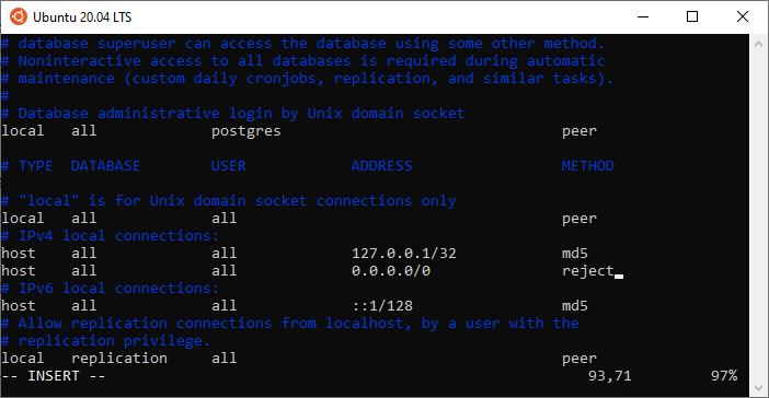PostgreSql Configurations (pg_hba.conf)Optional Step 2: you might want to configure PostgreSql to start automatically whenever you boot. To do this:

sudo update-rc.d postgresql enable

2. Apache Airflow Installation

We will install Airflow and its dependencies using pip:

pip install apache-airflow['postgresql']  
pip install psycopg2

By now you should have Airflow installed. By default, Airflow gets installed to ~/.local/bin. Remember to run the following command:

export PATH=$PATH:/home/your_user/.local/bin/

This is required so that the system knows where to locate Airflow’s binary.

Note: for this example we are not using virtualenv or Pipenv, but you can feel free to use it. Just make sure that environment dependencies are properly mapped when you setup Airflow to run as a service :)

3. Apache Airflow Configuration

Now we need to configure Airflow to use LocalExecutor and to use our PostgreSql database.

Go to Airflow’s installation directory and edit airflow.cfg.

vim airflow.cfg

Make sure that the executor parameter is set to LocalExecutor and SqlAlchemy connection string is set accordingly:

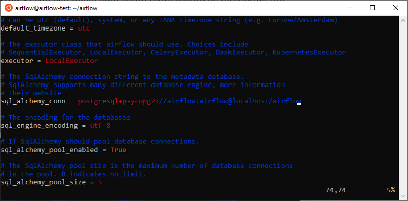Airflow configuration for LocalExecutorFinally, we need to initialize our database:

airflow initdb

Make sure that no error messages were displayed as part of initdb’s output.

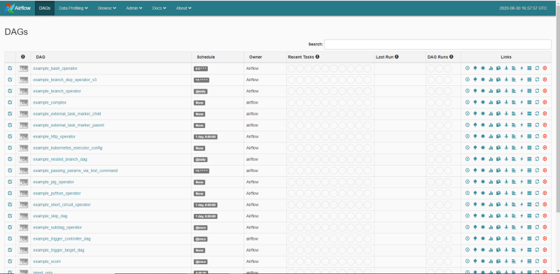
4. Testing

It is time to check if Airflow is properly working. To do that, we spin up the Scheduler and the Webserver:

airflow scheduler  
airflow webserver

Once you fire up your browser and point to your machine’s IP, you should see a fresh Airflow installation:

#### 5. Setting up Airflow to Run as a Service

Our last step is to configure the daemon for the Scheduler and the Webserver services. This is required so that we ensure that Airflow gets automatically restarted in case there is a failure, or after our machine is rebooted.

As an initial step, we need to configure Gunicorn. Since by default it is not installed globally, we need to create a symbolic link for it.

sudo ln -fs $(which gunicorn) /bin/gunicorn

Next, we create service files for Webserver and Scheduler:

sudo touch /etc/systemd/system/airflow-webserver.service  
sudo touch /etc/systemd/system/airflow-scheduler.service

Our airflow-webserver.service must look like the following:

#  
# Licensed to the Apache Software Foundation (ASF) under one  
# or more contributor license agreements. See the NOTICE file  
# distributed with this work for additional information  
# regarding copyright ownership. The ASF licenses this file  
# to you under the Apache License, Version 2.0 (the  
# “License”); you may not use this file except in compliance  
# with the License. You may obtain a copy of the License at  
#  
# <http://www.apache.org/licenses/LICENSE-2.0>  
#  
# Unless required by applicable law or agreed to in writing,  
# software distributed under the License is distributed on an  
# “AS IS” BASIS, WITHOUT WARRANTIES OR CONDITIONS OF ANY  
# KIND, either express or implied. See the License for the  
# specific language governing permissions and limitations  
# under the License.

[Unit]  
Description=Airflow webserver daemon  
After=network.target postgresql.service mysql.service  
Wants=postgresql.service mysql.service  
[Service]  
EnvironmentFile=/etc/environment  
User=airflow  
Group=airflow  
Type=simple  
ExecStart= /home/airflow/.local/bin/airflow webserver  
Restart=on-failure  
RestartSec=5s  
PrivateTmp=true  
[Install]  
WantedBy=multi-user.target

Similarly, we add the following content to airflow-scheduler.service:

#  
# Licensed to the Apache Software Foundation (ASF) under one  
# or more contributor license agreements. See the NOTICE file  
# distributed with this work for additional information  
# regarding copyright ownership. The ASF licenses this file  
# to you under the Apache License, Version 2.0 (the  
# “License”); you may not use this file except in compliance  
# with the License. You may obtain a copy of the License at  
#  
# <http://www.apache.org/licenses/LICENSE-2.0>  
#  
# Unless required by applicable law or agreed to in writing,  
# software distributed under the License is distributed on an  
# “AS IS” BASIS, WITHOUT WARRANTIES OR CONDITIONS OF ANY  
# KIND, either express or implied. See the License for the  
# specific language governing permissions and limitations  
# under the License.

[Unit]  
Description=Airflow scheduler daemon  
After=network.target postgresql.service mysql.service  
Wants=postgresql.service mysql.service  
[Service]  
EnvironmentFile=/etc/environment  
User=airflow  
Group=airflow  
Type=simple  
ExecStart=/home/airflow/.local/bin/airflow scheduler  
Restart=always  
RestartSec=5s  
[Install]  
WantedBy=multi-user.target

Note: depending on the directory where you installed Airflow, your ExecStart variable might need to be changed.

Now we just need to reload our system daemon, enable and start our services:

sudo systemctl daemon-reload  
sudo systemctl enable airflow-scheduler.service  
sudo systemctl start airflow-scheduler.service  
sudo systemctl enable airflow-webserver.service  
sudo systemctl start airflow-webserver.service

Our services should have been started successfully. To confirm that:

$ sudo systemctl status airflow-webserver.service  
$ sudo systemctl status airflow-scheduler.service

You should see some output stating that both services are active and enabled. For example, for the Webserver, you should see something similar to this:

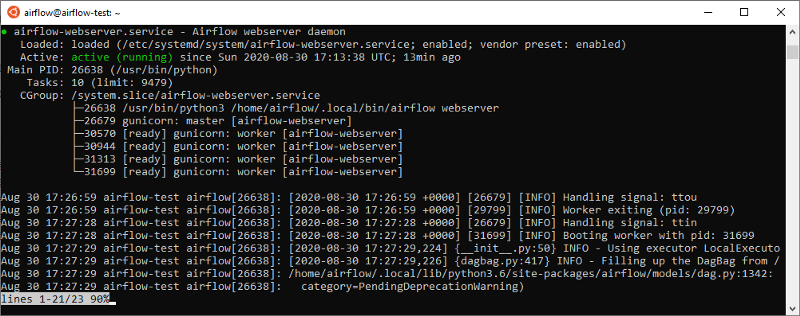That’s it. Now you have a basic Production setup for Apache Airflow using the LocalExecutor, which allows you to run DAGs containing parallel tasks and/or run multiple DAGs at the same time. This is definitely a must-have for any kind of serious use case — which I also plan on showcasing on a future post.

Of course, there are many possible improvements here:

• The most obvious one would be to automate these steps by creating a CICD pipeline with an Ansible runbook, for instance
• Using more secure PostgreSql credentials for Airflow and storing them in a more secure manner. We could store them as a secret variable within a CICD pipeline and set them up as environment variables, instead of storing in airflow.cfg
• Restricting permissions for Airflow users in both OS and PostgreSql

But for now, we will leave these steps for a future article.

I’m glad that you made it until here and I hope you found it useful. Check out my other articles:

Keeping Your Machine Learning Models on the Right Track: Getting Started with MLflow, Part 2
Learn how to use MLflow Model Registry to track, register and deploy Machine Learning Models effectively.mlopshowto.comKeeping Your Machine Learning Models on the Right Track: Getting Started with MLflow, Part 1
Learn why Model Tracking and MLflow are critical for a successful machine learning projectmlopshowto.comA Journey Into Machine Learning Observability with Prometheus and Grafana, Part I
Deploying Prometheus and Grafana on Kubernetes in 10 minutes for basic infrastructure monitoringmlopshowto.com

Data Pipeline Orchestration on Steroids: Getting Started with Apache Airflow, Part 1

Source: Unsplash### What is Apache Airflow?

Source: UnsplashApache Airflow is an open source data workflow management project originally created at AirBnb in 2014. In terms of data workflows it covers, we can think about the following sample use cases:

🚀 Automate Training, Testing and Deploying a Machine Learning Model

🍽 Ingesting Data from Multiple REST APIs

🚦 Coordinating Extraction, Transformation and Loading (ETL) or Extraction, Loading and Transformation (ELT) Processes Across an Enterprise Data Lake

As we can see, one of the main features of Airflow is its flexibility: it can be used for many different data workflow scenarios. Due to this aspect and to its rich feature set, it has gained significant traction over the years, having been battle tested in many companies, from startups to Fortune 500 enterprises. Some examples include Spotify, Twitter, Walmart, Slack, Robinhood, Reddit, PayPal, Lyft, and of course, AirBnb.

OK, But Why?

Feature Set

• Apache Airflow works with the concept of Directed Acyclic Graphs (DAGs), which are a powerful way of defining dependencies across different types of tasks. In Apache Airflow, DAGs are developed in Python, which unlocks many interesting features from software engineering: modularity, reusability, readability, among others.

Source: Apache Airflow Documentation* Sensors, Hooksand Operatorsare the main building blocks of Apache Airflow. They provide an easy and flexible way of connecting to multiple external resources. Want to integrate with Amazon S3? Maybe you also want to add Azure Container Instances to the picture in order to run some short-lived Docker containers? Perhaps running a batch workload in an Apache Spark or Databricks cluster? Or maybe just executing some basic Python code to connect with REST APIs? Airflow ships with multiple operators, hooks and sensors out of the box, which allow for easy integration with these resources, and many more, such as: DockerOperator, BashOperator, HiveOperator, JDBCOperator— the list goes on.You can also build upon one of the standard operators and create your own. Or you can simply write your own operators, hooks and sensors from scratch.

• The UI allows for quick and easy monitoring and management of your Airflow instance. Detailed logs also make it easier to debug your DAGs.

Airflow UI Tree View. Source: Airflow Documentation…and there are many more. Personally, I believe one of the fun parts of working with Airflow is discovering new and exciting features as you use it — and if you miss something, you might as well create it.

• It is part of the Apache Foundation, and the community behind it is pretty active — currently there are more than a hundred direct contributors. One might argue that Open Source projects always run the risk of dying at some point — but with a vibrant developer community we can say this risk is mitigated. In fact, 2020 has seen individual contributions for Airflow at an all-time high.

Apache Airflow Tutorial

Time to get our hands dirty and actually start with the tutorial.

There are multiple ways of installing Apache Airflow. In this introduction we will cover the easiest one, which is by installing it from the PyPi repository.

Basic Requirements

• Python 3.6+
• Pip
• Linux/Mac OS — for those running Windows, activate and installWindows Subsystem for Linux (WSL), download Ubuntu 18 LTS from the Windows Marketplace and be happy :)

Initial Setup

• Create a new directory for your Airflow project (e.g. “airflow-intro”)
• From your new directory, create and activate a new virtual environment for your Airflow project using venv

# Run this from newly created directory to create the venv  
python3 -m venv venv

# Activate your venv  
source venv/bin/activate

• Install apache-airflow through pip

pip install apache-airflow

Before proceeding, it is important to discuss a bit about Airflow’s main component: the Executor. The name is pretty self-explanatory: this component handles the coordination and execution of different tasks across multiple DAGs.

There are many types of Executors in Apache Airflow, such as the SequentialExecutor, LocalExecutor, CeleryExecutor, DaskExecutor and others. For the sake of this tutorial, we will focus on the SequentialExecutor. It presents very basic functionality and has a main limitation, which is the fact that it cannot execute tasks in parallel. This is due to the fact that it leverages a SQLite database as the backend (which can only handle one connection at a time), hence multithreading is not supported. Therefore it is not recommended for a Production setup, but it should not be an issue for our case.

Going back to our example, we need to initialize our backend database. But before that, we must override our AIRFLOW_HOME environment variable, so that we specify that our current directory will be used for running Airflow.

export AIRFLOW\_HOME=$(pwd)

Now we can initialize our Airflow database. We can do this by simply executing the following:

airflow initdb

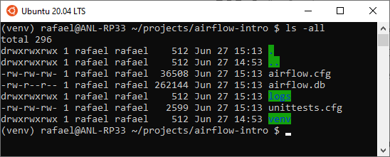
Take a look at the output and make sure that no error messages are displayed. If everything went well, you should now see the following files in your directory:

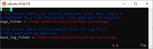
* To confirm if the initialization is correct, quickly inspect airflow.cfg and confirm if the following lines correctly point to your work directory in the [core] section. If they do, you should be good to go.

Optional: Airflow ships with many sample DAGs, which might help you get up to speed with how they work. While it is certainly helpful, it can make your UI convoluted. You can set load_examples to False, so that you will see only your own DAGs in the Airflow’s UI.

DAG Creation

We will start with a really basic DAG, which will do two simple tasks:

1. Create a text file
2. Rename this text file

To get started, create a new Python script file named simple_bash_dag.py inside your dags folder. In this script, we must first import some modules:

# Python standard modules  
from datetime import datetime, timedelta

# Airflow modules  
from airflow import DAG  
from airflow.operators.bash\_operator import BashOperator

We now proceed to creating a DAG object. In order to do that, we must specify some basic parameters, such as: when will it become active, which intervals do we want it to run, how many retries should be made in case any of its tasks fail, and others. So let’s define these parameters:

default\_args = {  
    'owner': 'airflow',  
    'depends\_on\_past': False,  
    # Start on 27th of June, 2020  
    'start\_date': datetime(2020, 6, 27),  
    'email': ['airflow@example.com'],  
    'email\_on\_failure': False,  
    'email\_on\_retry': False,  
    # In case of errors, do one retry  
    'retries': 1,  
    # Do the retry with 30 seconds delay after the error  
    'retry\_delay': timedelta(seconds=30),  
    # Run once every 15 minutes  
    'schedule\_interval': '\*/15 \* \* \* \*'  
}

We have defined our parameters. Now it is time to actually tell our DAG what it is supposed to do. We do this by declaring different tasks — T1 and T2. We must also define which task depends on the other.

with DAG(

    dag\_id=’simple\_bash\_dag’,  
    default\_args=default\_args,  
    schedule\_interval=None,  
    tags=[‘my\_dags’],  
) as dag:

    #Here we define our first task  
    t1 = BashOperator(bash\_command=”touch ~/my\_bash\_file.txt”, task\_id=”create\_file”)

    #Here we define our second task  
    t2 = BashOperator(bash\_command=”mv ~/my\_bash\_file.txt ~/my\_bash\_file\_changed.txt”, task\_id=”change\_file\_name”)

    # Configure T2 to be dependent on T1’s execution  
    t1 >> t2

And as simple as that, we have finished creating our DAG 🎉

Testing our DAG

Let’s see how our DAG looks like and most importantly, see if it works.

To do this, we must start two Airflow components:

• The Scheduler, which controls the flow of our DAGs

airflow scheduler

• The Web Server, an UI which allows us to control and monitor our DAGs

airflow webserver

You should see the following outputs (or at least something similar):

Output for the Scheduler’s startup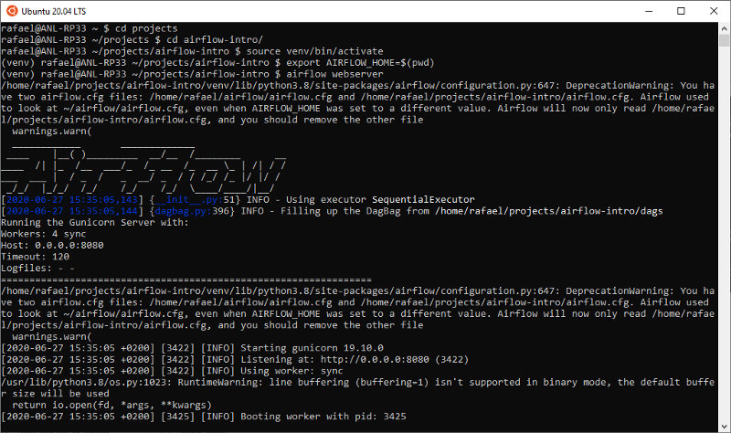Output for the Webserver’s startup#### Showtime

We should now be ready to look at our Airflow UI and test our DAG.

Just fire up your navigator and go to https://localhost:8080. Once you hit Enter, the Airflow UI should be displayed.

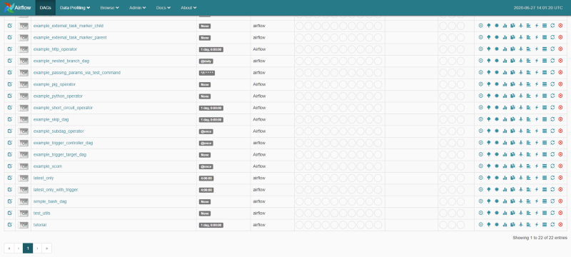Look for our DAG — simple_bash_dag — and click on the button to its left, so that it is activated. Last, on the right hand side, click on the play button ▶ to trigger the DAG manually.

Clicking on the DAG enables us to see the status of the latest runs. If we click on the Graph View, we should see a graphical representation of our DAG — along with the color codes indicating the execution status for each task.

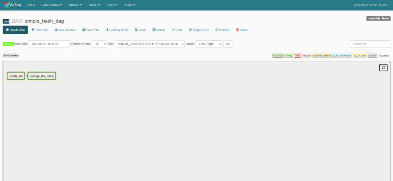As we can see, our DAG has run successfully 🍾

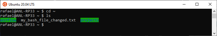
We can also confirm that by looking at our home directory:

### Wrap Up

• We had a quick tutorial about Apache Airflow, how it is used in different companies and how it can help us in setting up different types of data pipelines
• We were able to install, setup and run a simple Airflow environment using a SQLite backend and the SequentialExecutor
• We used the BashOperator to run simple file creation and manipulation logic

There are many nice things you can do with Apache Airflow, and I hope my post helped you get started. If you have any questions or suggestions, feel free to comment.

You might also like some of my other stories:

Keeping Your Machine Learning Models on the Right Track: Getting Started with MLflow, Part 2
Learn how to use MLflow Model Registry to track, register and deploy Machine Learning Models effectively.mlopshowto.comKeeping Your Machine Learning Models on the Right Track: Getting Started with MLflow, Part 1
Learn why Model Tracking and MLflow are critical for a successful machine learning projectmlopshowto.comAn Apache Airflow MVP: Complete Guide for a Basic Production Installation Using LocalExecutor
Simple and quick way to bootstrap Airflow in productiontowardsdatascience.co

Deep Blue Sea: Using Deep Learning to Detect Hundreds of Different Plankton Species

In this post, we will go through a pipeline for using Keras, Deep Learning, Transfer Learning and Ensemble Learning to predict the species from hundreds of plankton species

Source: UnsplashBack in 2014, Booz Allen Hamilton and the Hartfield Marine Center at the Oregon State University organized a fantastic Data Science Kaggle Competition as part of that year’s National Data Science Bowl.

The objective of the competition was to create an algorithm for automatically classifying different plankton images as one among 121 different species. From the competition’s home page:

Traditional methods for measuring and monitoring plankton populations are time consuming and cannot scale to the granularity or scope necessary for large-scale studies. Improved approaches are needed. One such approach is through the use of an underwater imagery sensor. This towed, underwater camera system captures microscopic, high-resolution images over large study areas. The images can then be analyzed to assess species populations and distributions.

The National Data Science Bowl challenges you to build an algorithm to automate the image identification process. Scientists at the Hatfield Marine Science Center and beyond will use the algorithms you create to study marine food webs, fisheries, ocean conservation, and more. This is your chance to contribute to the health of the world’s oceans, one plankton at a time.

As part of a graduate Machine Learning course at the University of Amsterdam, students were tasked with this challenge. My team’s model finished in 3rd place among 30 other teams, with an accuracy score of 77.6% — a difference of ~0.005 between our score and the winning team.

I decided to share a bit of our strategy, our model, challenges and tools we used. We will go through the items below:

1. Deep Neural Networks: Recap
2. Convolutional Neural Networks: Recap
3. Activation Functions
4. Data at a Glance
5. Data Augmentation Techniques
6. Transfer Learning
7. Ensemble or Stacking
8. Putting it All Together

Deep Neural Networks

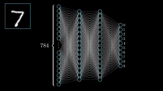Source: 3Blue1BrownI will go ahead and assume that you are already familiar with the concept of Artificial Neural Networks (ANN). If that is the case, the concept of Deep Neural Networks is fairly simple. If that is not the case, this video has a great and detailed explanation about how it works. Finally, you can check out this specialization created by the great Andrew Ng if you want to gain an edge on Deep Learning.

Deep Neural Networks (DNN) are a specific group of ANNs that are characterised by having a significant amount of hidden layers, among other aspects.

The fact that DNNs have many layers allows them to perform well in classification or regression tasks involving pattern recognition problems within complex, unstructured data, such as image, video and audio recognition.

Convolutional Neural Networks

Convolutional Neural Networks (CNNs) are a specific architecture type of DNNs which add the concept of Convolutional Layers. These layers are extremely important to extract relevant features from images to perform image classification.

This is done by applying different kinds of transformations across each of the image’s RGB channels. So in layman terms, we can say that Convolution operations perform transformations over image channels in order to make it easier for a neural network to detect certain patterns.

While getting into the theoretical and mathematical details about Convolutional Layers is beyond the scope of this post, I can recommend this chapter from a landmark book on Deep Learning by Goodfellow et al to better understand not only Convolution Layers, but all aspects related to Deep Learning. For those who want to get their hands dirty, this course from deeplearning.ai is also great for getting a head start into Convolutional Neural Networks with Python and Tensorflow.

Activation Functions

Activation functions are also important in this context, and in the case of DNNs, some of the activation functions that are commonly used are ReLU, tanh, PReLU, LReLU, Softmax and others.

These functions represented a huge shift from classical ANNs, which used to rely on the Sigmoid function for activation. This type of activation function is known to suffer from the Vanishing Gradient problem; rectifying functions such as ReLU present one of the possible solutions for this issue.

Data at a Glance

Now going back to our problem. The data is composed by training and testing sets. In the training set, there are ~24K images of plankton and in the testing set there are ~6K images of plankton.

A first look at the data shows that we have an imbalanced dataset — the plot below shows how many images from each species we have in the training set.

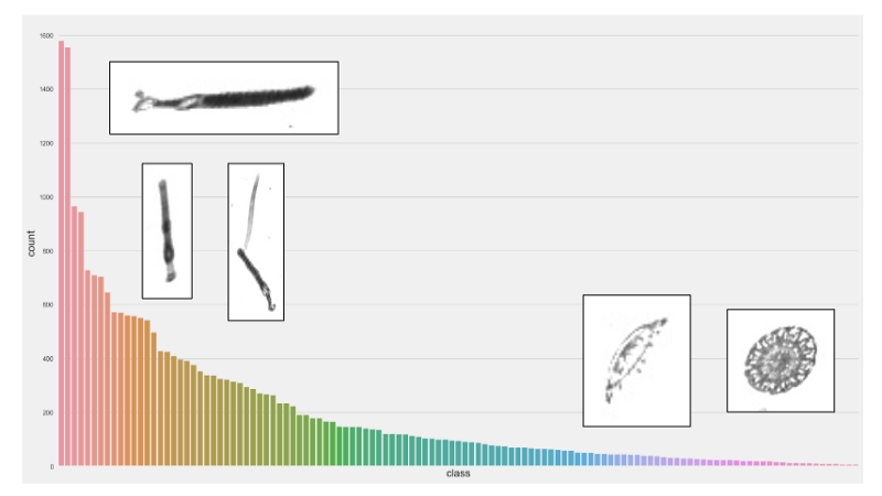Number of images in the dataset for different plankton species. Source: AuthorThis is a problem, specially for species that are under represented. Most likely our model would not have enough training data to be able to detect plankton images from these classes.

The approach we used to tackle this problem was to set class weights for imbalanced classes. Basically, if we have image classes A and B, where A is underrepresented and B is overrepresented, we could want to treat every instance of class A as 50 instances of class B.

Thismeans that in our loss function, we assign higher value to these instances. Hence, the loss becomes a weighted average, where the weight of each sample is specified by class_weight and its corresponding class.

Data Augmentation

One of the possible caveats of Deep Learning is that it usually requires huge amounts of training samples to achieve a good performance. A common approach for dealing with a small training set is augmenting it.

This can be done by generating artificial samples for one or more classes in the dataset by rotating, zooming, mirroring, blurring or shearing the original set of images.

In our case, we used the Keras Preprocessing library to perform online image augmentation — transformation was performed on a batch-by-batch basis as soon as each batch was loaded through the Keras ImageDataGenerator class.

Transfer Learning

One of the first decisions one needs to make when tackling an image recognition problem is whether to use an existing CNN architecture or creating a new one.

Our first shot at this problem involved coming up with a new CNN architecture from scratch, which we called SimpleCNN. The accuracy obtained with this architecture was modest — 60%.

With lots of researchers constantly working throughout the world in different architectures, soon we realised that it would be infeasible to come up with a new architecture that could be better than an existing one, without spending significant amounts of time and computing power training it and testing it.

With this in mind, we decided to leverage the power of Transfer Learning.

The basic idea of Transfer Learning is using existing pre-trained, established CNN architectures (and weights, if needed) for a particular prediction task.

Most deep learning platforms such as Keras and PyTorch have out of the box functionality for doing that. By using Transfer Learning, we obtained models with accuracies between 71% and 74%.

Ensemble Learning

We obtained a fairly good accuracy with Transfer Learning, but we still weren’t satisfied. So we decided to use all the models we trained at the same time.

One approach that is commonly used by most successful Kaggle teams is to train separate models and create an ensemble with the best performing ones.

This is ideal, as it allows team members to work in parallel. But the main intuition behind this idea is that predictions from an individual model could be biased; by using multiple predictions from an ensemble, we are getting a collegiate opinion, similar to a voting process for making a decision. In Ensemble Learning, we can have Hard Voting or Soft Voting.

Source: UnsplashWe opted for Hard Voting. The main difference between the two is that while in the first we perform a simple majority vote taking predicted classes into consideration, in the second we take an average of the probabilities predicted by each model for each class, selecting the most likely one in the end.

Putting it all Together

After putting all the pieces together, we obtained a model with a ~77.6% accuracy score for predicting plankton species for 121 distinct classes.

The diagram below shows not only the different architectures that were individually trained and became part of our final stack, but also a high level perspective of all the steps we conducted for our prediction pipeline.

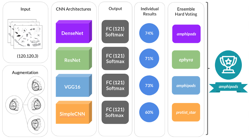A diagram showing the preprocessing, CNN architecture, training and ensembling aspects of our pipeline. Source: Author### Conclusions & Final Remarks

• Transfer Learning is excellent for optimizing time-to-market for new data products and platforms, while being really straightforward.
• Ensemble Learning was also important from an accuracy standpoint — but would probably present its own challenges in an online, real-world, production environment scenario
• As with most Data Science problems, data augmentation & feature engineering were key for getting good results

For similar problems in the future, we would try to:

• Explore a bit of offline image augmentation with libraries such as skimage and OpenCV
• Feed some basic image features such as width, height, pixel intensity and others to Keras’ Functional API

But this will be subject for a next post. In the meantime, check my other stories:

Keeping Your Machine Learning Models on the Right Track: Getting Started with MLflow, Part 2
Learn how to use MLflow Model Registry to track, register and deploy Machine Learning Models effectively.mlopshowto.comData Pipeline Orchestration on Steroids: Getting Started with Apache Airflow, Part 1
What is Apache Airflow?towardsdatascience.comData Leakage, Part I: Think You Have a Great Machine Learning Model? Think Again
Got insanely excellent metric scores for your classification or regression model? Chances are you have data leakage.towardsdatascience.com

Data Leakage, Part I: Think You Have a Great Machine Learning Model? Think Again

Got insanely excellent metric scores for your classification or regression model? Chances are you have data leakage.

In this post, you will learn:

• What is data leakage
• How to detect it and
• How to avoid it

You were presented with a challenging problem.

As a driven, gritty, aspiring data scientist, you used all tools that were within your reach.

You gathered a reasonable amount of data. You have got a considerable amount of features. You were even able to come up with many additional features through feature engineering.

You used the fanciest possible machine learning model. You made sure your model didn’t overfit. You properly split your dataset in training and test sets.

You even used K-Folds validation.

You had been cracking your head for some time, and it seems that you finally had that “aha” moment.

Chances are data leakage took on you.You were able to get an impressive 99% AUC (Area Under Curve) score for your classification problem. Your model has outstanding results when it comes to predicting labels for your testing set, properly detecting True Positives, True Negatives, False Positives and False Negatives.

Or, in the case you had a regression problem, your model was able to get excellent MAE (Mean Absolute Error), MSE (Mean Squared Error) and R2 (Coefficient of Determination) scores.

Congratulations!

Good job, you got zero error! NOT### Too Good to be True?

As a result of your efforts and the results you obtained, everyone at the office admires you. You have been lauded as the next machine learning genius.

You can even picture yourself in your next vacation driving a convertible.

But before that, it is time for showdown: your model is going into production.

However, when it’s finally time for your model to start doing some perfect predictions out on the wild, something weird happens.

Your model is simply not good enough.

What is Data Leakage

Data Leakage happens when for some reason, your model learns from data that wouldn’t (or shouldn’t) be available in a real-world scenario.

Or, in other words:

When the data you are using to train a machine learning algorithm happens to have the information you are trying to predict.

— Daniel Gutierrez, Ask a Data Scientist: Data Leakage

How to Detect Data Leakage

Data Leakage happens a lot when we are dealing with data that has Time Series characteristics. That is, we have a series of data points that are distributed chronologically.

One of the rules of thumb for trying to avoid Data Leakage for time series data is performing cross validation.

Cross validation involves randomly selecting data points from your dataset and assigning them to training and testing sets. Data preparation and feature engineering steps are done separately for the training and testing sets.

Nevertheless, depending on the nature of your dataset, you could have a target variable with a distribution that is similar for both training and testing sets.

In such case, it is easy for a model to learn that depending on the moment in time, probabilities for each target variable class change accordingly.

As a result, any feature from the dataset that has a relationship with time could potentially lead to data leakage.

How to Avoid Data Leakage

There is no silver bullet for avoiding data leakage.

It requires a change of mindset.

But the first step, in case you have a time-series dataset, is removing time-related features.

Remove Time-Related Features

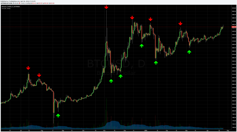Time series analysis for Bitcoin prices.Typical forecasting problems, such as weather, cryptocurrencies and stock market price prediction require time series data analysis.

You might feel tempted to remove time-related features from your dataset. However, depending on the number of features in your dataset, this could prove to be a more complicated task, and you might end up removing features that could benefit your model.

On the other hand, incremental ID fields don’t add predictive power to your model and could cause data leakage. Hence most of the time it is recommended to remove them from your dataset.

But apart from that, tackling data leakage involves more of a mindset change when it comes to cross validation rather than feature selection.

Nested Cross-Validation

Source: https://sebastianraschka.com/faq/docs/evaluate-a-model.htmlNested Cross Validation is the most appropriate method to evaluate performance when conceptualizing a predictive model for time-series data.

One basic way of performing nested cross validation is predicting the second half. This involves the following steps:

1. For a particular time-series dataset, select a point p in time
2. All data points before p will be part of the training set
3. All remaining data points after p will be part of the testing set

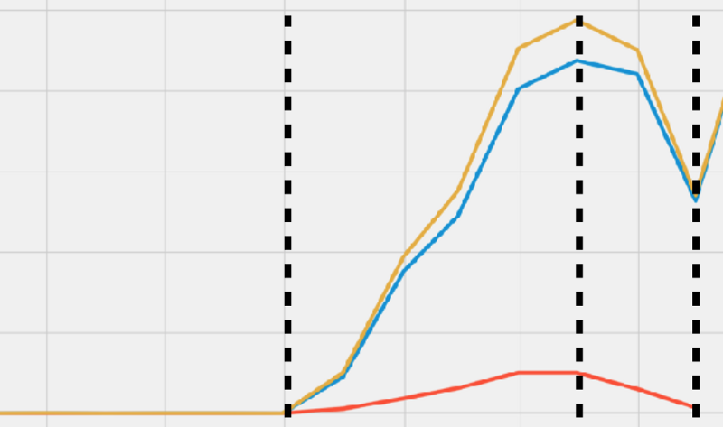In this example, we perform the model training for the first portion of the dataset that is between the two dotted lines, and model testing for the second portion to the right.Predicting the second half is an easy and straightforward nested cross validation method for avoiding data leakage. It is also closer to the real-word, production scenario, but it comes with some caveats.

Depending on the splitting approach, bias could be introduced, and as a result, biased estimates of prediction error could be produced for an independent dataset.

This is where forward chaining comes to the rescue.

Forward chaining involves creating many different folds within your dataset, in a way that you predict the second half for each of these folds.

This exposes the model to different points in time, thus mitigating bias. But this is subject for a next post.

In this article you learned:

• What is data leakage and why it could be a problem for you
• How to detect data leakage
• How to avoid data leakage — by removing time-related features and performing nested cross validation

You Might Also Like

Keeping Your Machine Learning Models on the Right Track: Getting Started with MLflow, Part 2
Learn how to use MLflow Model Registry to track, register and deploy Machine Learning Models effectively.mlopshowto.comKeeping Your Machine Learning Models on the Right Track: Getting Started with MLflow, Part 1
Learn why Model Tracking and MLflow are critical for a successful machine learning projectmlopshowto.comData Pipeline Orchestration on Steroids: Getting Started with Apache Airflow, Part 1
What is Apache Airflow?towardsdatascience.com

A Gentle Introduction to Credit Risk Modeling with Data Science - Part 2

In this post, we will use Data Science and Exploratory Data Analysis to understand how borrower variables such as income, job title and employment length affect credit risk.

Understanding how borrowers financials affect credit risk

“You are the Ninja Generation. No income. No job. No Assets.”In our last post, we started using Data Science for Credit Risk Modeling by analyzing loan data from Lending Club.

We’ve raised some possible indications that the loan grades assigned by Lending Club are not as optimal as possible.

Over the next posts, our objective will be using Machine Learning to beat those loan grades.

We will do this by conceptualizing a new credit score predictive model in order to predict loan grades.

In this post, we will use Data Science and Exploratory Data Analysis to delve deeper into some of the Borrower Variables, such as annual income and employment status and see how they affect other variables.

This is crucial to help us visualize and understand what kind of public are we dealing with, allowing us to come up with an Economic Profile.

Economic Profile

In the dataset, we have some variables from each borrower’s economic profile, such as:

• Income: annual income in USD
• Employment Length: how many years of employment at the current job.
• Employment Title: job title provided by the borrower in the loan application

We will analyze each of these variables and how they interact within our dataset.

Show me the Money

We have two variables reflecting borrowers’ income, depending on the nature of the application: single annual income or joint annual income.

Single applications are the ones filed by only one person, while joint applications are filed by two or more people.

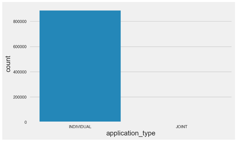As it can be seen in the countplot above, the quantity of joint applications is negligible.

Let’s generate a couple of violin plots and analyze the annual income for single and joint applications together.

Violin plots are similar to box plots, except that they also show the probability density of the data at different values (in the simplest case this could be a histogram).

Our first violin plot looks weird.

Before digging deeper, let’s zoom in and try to understand why it has this format by generating a distribution plot for annual incomes from single applications.

Annual Incomes for Single Applications

We can observe a few particularities:

• It is heavily skewed —deviates from the gaussian distribution.
• It is heavily peaked.
• It has a long right tail.

These aspects are usually observed in distributions which are fit by a Power Law.

A power law is a functional relationship between two quantities, where a relative change in one quantity results in a proportional relative change in the other quantity, independent of the initial size of those quantities: one quantity varies as a power of another.

Throughout the years, some scientists have analyzed a variety of distributions. There is reasonable amount of work indicating that some of these distributions could be fit by a Power Law, such as:

• Annual Income in Some Countries
• American Individuals’ Net Worth
• City Populations
• Species Extinction
• Species Body Mass
• Sizes of Craters on the Moon
• Words in Most Language Corpi

For our dataset, if we only consider employed individuals (or income greater than zero), we could very informally say that we have a Power Law candidate distribution — this would be in line with the first paper referenced above (Distributions of Korean Household Incomes).

However, formally proving a distribution’s goodness-of-fit is not a trivial task and thus would require a reasonable amount of work, which is outside the scope of this article. If you’re interested into this subject, check out this excellent paper from Aaron Clauset.

Coming back to our problem, let’s zoom into the distribution for annual joint incomes and see how they differ from the annual single incomes data distribution.

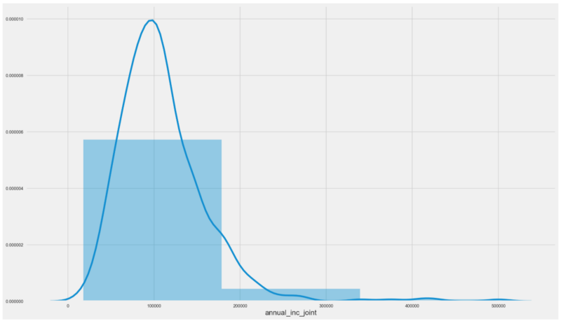Interestingly enough, we have a different animal here.

Our distribution is unimodal and resembles the gaussian distribution, beingskewed to the left.

Income versus Loan Amount

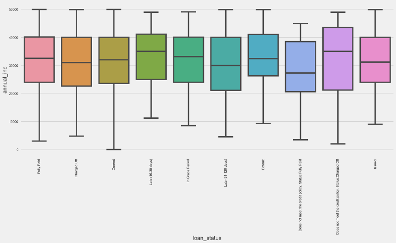
We will check the relationship between Income and Loan Amount by generating a boxplot.

But in order to do this we’ll look at a subset from our data, where income is less than USD 120K per year.

The reason for this is that applications with income above this limit are quite not statistically representative in our population — from 880K loans, only 10% have annual incomes higher than USD 120K.

If we don’t cap our annual income, we would have a lot of outliers and our boxplot would look like the one on the left:

From the right side boxplot, we have a few highlights:

• Fully Paid status quartile distribution is very different from Charged Off. Moreover, it is similar to Current, In Grade Period and Issued. Intuitively, this leads us to think that Lending Club has been more selective with its newer loans.
• Charged Off and Default statuses hold similarities in terms of the quartile distribution, differing from all the others.

This looks like good news in terms of importance of the income variable for predicting loan grades.

Will these variables represent critical information for our model?

Let’s add one more dimension to the analysis by generating the boxplots for Income versus Loan Grade.

Unsurprisingly, A graded loans have a median income that is superior to other grades, and the same can be said about the other quartiles.

Note however that F, G and B graded loans hold a similar income quartile distribution, lacking consistency.

Perhaps income is not that critical when determining LC’s loan grades?

We will find that later.

Employment Title

While annual income gives a good indication on the financial situation of each of the borrowers, employment title can also give us some valuable insights. Some professions have a higher turnover, are riskier or more stressful than others, which might impact borrowers financial capacity.

Let’s start by generating a count plot for employment titles considering annual income lower than USD 120K.

Most applications have a null employment title. Other than that, top 5 occupations for this subset are:

1. Teacher
2. Manager
3. Registered Nurse
4. RN (possibly Registered Nurse)
5. Supervisor

Having a lot of applications with “None” as employment title could be reason for concern. This could be explained by some possible scenarios, among them:

• Unemployed people are getting loans
• Some of the applications are being filed without this information

Let’s investigate this further by checking the annual income from people with “None” as employment title.

All the quartiles seem to be a little bit above zero, which wouldn’t be a surprise.

But there are also a lot of outliers — some people with no employment title and an annual income of more than USD 250K, for example.

Maybe Compliance and KYC are not doing a good job?

At this point, we don’t know.

Before answering this question, let me introduce you to NINJA Loans.

NINJA Loans

In financial markets, NINJA Loan is a slang term for a loan extended to a borrower with “no income, no job and no assets.” Whereas most lenders require the borrower to show a stable stream of income or sufficient collateral, a NINJA loan ignores the verification process.

Let’s see if the applications with no income have actually got a loan.

We can conclude that many people with almost zero annual income actually got loans.

At the same time, there are current loans which were granted to people with zero annual income.

Bottomline for now is that we can’t safely assume this is a problem with Compliance or KYC. This scenario could also relate to LC’s risk appetite, or simply bad data.

But there is some indication that LC’s risk appetite has been steadily growing, since some of the current loans were accepted without any annual income.

The Good, the Bad and the Wealthy

Just out of curiosity, let’s check the employment titles for individuals with an annual income that is superior to USD 120K.

Again, most of the applications within this subset don’t have an employment title. For the rest of them, top 5 positions by frequency are:

1. Director
2. Manager
3. Vice President
4. Owner
5. President

We can see that we have more senior level positions as well as high level self-employed professionals such as attorneys and physicians. No surprises here either.

We must remember that this subset represents around 80K loans, which stands for less than 10% of the entire population.

Time is Money

From a P2P loan investor strategy, it is important to understand the size of the cash flows (income amount) and the stability. Employment length can be a good proxy for that.

However, it is known that employment length is self reported by LC loan applicants. Lending Club does not verify it.

So the question is — is it reliable as a credit risk predictor?

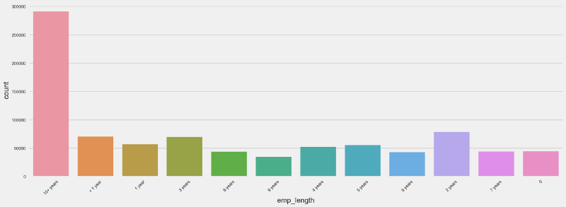
From the count plot below, we can see that we have many applications where the borrower has more than 10 years of employment tenure.

Let’s see how employment length correlates with the loan status.

Since we’re talking about two categorical variables, we will generate some dummy variables and see how the pearson correlation between them looks like through a heatmap.

Unfortunately, there are no significant linear correlations between the dummy variables related to employment length and loan status.

Would the correlations between employment length and the loan grade show a different story?

Same old — no absolute correlation scores above 0.4.

Our quest does not end here, though.

We will continue expanding our analysis in a next post, where we will analyze hybrid loan x borrower characteristics, such as debt to income ratio, delinquency rates, and also other types of data such as geographic data and macroeconomic variables.

Getting to understand this public will help us achieve our objective in the longer run, which is creating a new machine learning model for predicting loan grades and credit default.

You Might Also Like

Keeping Your Machine Learning Models on the Right Track: Getting Started with MLflow, Part 2
Learn how to use MLflow Model Registry to track, register and deploy Machine Learning Models effectively.mlopshowto.comKeeping Your Machine Learning Models on the Right Track: Getting Started with MLflow, Part 1
Learn why Model Tracking and MLflow are critical for a successful machine learning projectmlopshowto.comAbout MLOps And Why Most Machine Learning Projects Fail — Part 1
If you have been involved with Machine Learning (or you are aiming to be), you might be aware that reaping the…mlopshowto.com