A Gentle Introduction to Credit Risk Modeling with Data Science - Part 2

In this post, we will use Data Science and Exploratory Data Analysis to understand how borrower variables such as income, job title and employment length affect credit risk.

Understanding how borrowers financials affect credit risk

“You are the Ninja Generation. No income. No job. No Assets.”In our last post, we started using Data Science for Credit Risk Modeling by analyzing loan data from Lending Club.

We’ve raised some possible indications that the loan grades assigned by Lending Club are not as optimal as possible.

Over the next posts, our objective will be using Machine Learning to beat those loan grades.

We will do this by conceptualizing a new credit score predictive model in order to predict loan grades.

In this post, we will use Data Science and Exploratory Data Analysis to delve deeper into some of the Borrower Variables, such as annual income and employment status and see how they affect other variables.

This is crucial to help us visualize and understand what kind of public are we dealing with, allowing us to come up with an Economic Profile.

Economic Profile

In the dataset, we have some variables from each borrower’s economic profile, such as:

• Income: annual income in USD
• Employment Length: how many years of employment at the current job.
• Employment Title: job title provided by the borrower in the loan application

We will analyze each of these variables and how they interact within our dataset.

Show me the Money

We have two variables reflecting borrowers’ income, depending on the nature of the application: single annual income or joint annual income.

Single applications are the ones filed by only one person, while joint applications are filed by two or more people.

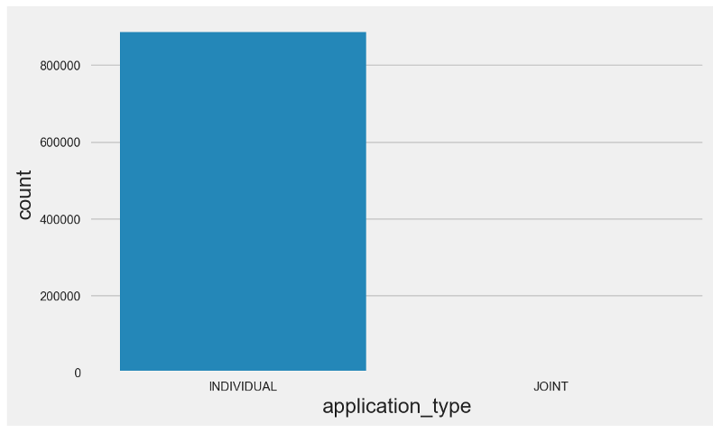As it can be seen in the countplot above, the quantity of joint applications is negligible.

Let’s generate a couple of violin plots and analyze the annual income for single and joint applications together.

Violin plots are similar to box plots, except that they also show the probability density of the data at different values (in the simplest case this could be a histogram).

Our first violin plot looks weird.

Before digging deeper, let’s zoom in and try to understand why it has this format by generating a distribution plot for annual incomes from single applications.

Annual Incomes for Single Applications

We can observe a few particularities:

• It is heavily skewed —deviates from the gaussian distribution.
• It is heavily peaked.
• It has a long right tail.

These aspects are usually observed in distributions which are fit by a Power Law.

A power law is a functional relationship between two quantities, where a relative change in one quantity results in a proportional relative change in the other quantity, independent of the initial size of those quantities: one quantity varies as a power of another.

Throughout the years, some scientists have analyzed a variety of distributions. There is reasonable amount of work indicating that some of these distributions could be fit by a Power Law, such as:

• Annual Income in Some Countries
• American Individuals’ Net Worth
• City Populations
• Species Extinction
• Species Body Mass
• Sizes of Craters on the Moon
• Words in Most Language Corpi

For our dataset, if we only consider employed individuals (or income greater than zero), we could very informally say that we have a Power Law candidate distribution — this would be in line with the first paper referenced above (Distributions of Korean Household Incomes).

However, formally proving a distribution’s goodness-of-fit is not a trivial task and thus would require a reasonable amount of work, which is outside the scope of this article. If you’re interested into this subject, check out this excellent paper from Aaron Clauset.

Coming back to our problem, let’s zoom into the distribution for annual joint incomes and see how they differ from the annual single incomes data distribution.

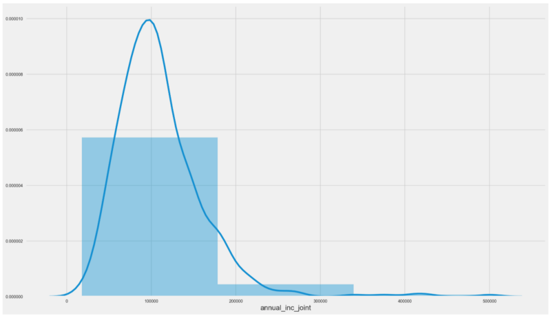Interestingly enough, we have a different animal here.

Our distribution is unimodal and resembles the gaussian distribution, beingskewed to the left.

Income versus Loan Amount

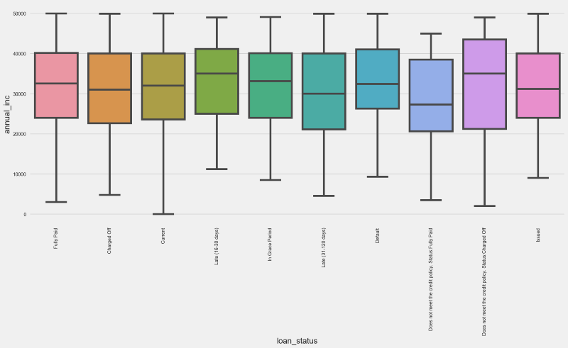
We will check the relationship between Income and Loan Amount by generating a boxplot.

But in order to do this we’ll look at a subset from our data, where income is less than USD 120K per year.

The reason for this is that applications with income above this limit are quite not statistically representative in our population — from 880K loans, only 10% have annual incomes higher than USD 120K.

If we don’t cap our annual income, we would have a lot of outliers and our boxplot would look like the one on the left:

From the right side boxplot, we have a few highlights:

• Fully Paid status quartile distribution is very different from Charged Off. Moreover, it is similar to Current, In Grade Period and Issued. Intuitively, this leads us to think that Lending Club has been more selective with its newer loans.
• Charged Off and Default statuses hold similarities in terms of the quartile distribution, differing from all the others.

This looks like good news in terms of importance of the income variable for predicting loan grades.

Will these variables represent critical information for our model?

Let’s add one more dimension to the analysis by generating the boxplots for Income versus Loan Grade.

Unsurprisingly, A graded loans have a median income that is superior to other grades, and the same can be said about the other quartiles.

Note however that F, G and B graded loans hold a similar income quartile distribution, lacking consistency.

Perhaps income is not that critical when determining LC’s loan grades?

We will find that later.

Employment Title

While annual income gives a good indication on the financial situation of each of the borrowers, employment title can also give us some valuable insights. Some professions have a higher turnover, are riskier or more stressful than others, which might impact borrowers financial capacity.

Let’s start by generating a count plot for employment titles considering annual income lower than USD 120K.

Most applications have a null employment title. Other than that, top 5 occupations for this subset are:

1. Teacher
2. Manager
3. Registered Nurse
4. RN (possibly Registered Nurse)
5. Supervisor

Having a lot of applications with “None” as employment title could be reason for concern. This could be explained by some possible scenarios, among them:

• Unemployed people are getting loans
• Some of the applications are being filed without this information

Let’s investigate this further by checking the annual income from people with “None” as employment title.

All the quartiles seem to be a little bit above zero, which wouldn’t be a surprise.

But there are also a lot of outliers — some people with no employment title and an annual income of more than USD 250K, for example.

Maybe Compliance and KYC are not doing a good job?

At this point, we don’t know.

Before answering this question, let me introduce you to NINJA Loans.

NINJA Loans

In financial markets, NINJA Loan is a slang term for a loan extended to a borrower with “no income, no job and no assets.” Whereas most lenders require the borrower to show a stable stream of income or sufficient collateral, a NINJA loan ignores the verification process.

Let’s see if the applications with no income have actually got a loan.

We can conclude that many people with almost zero annual income actually got loans.

At the same time, there are current loans which were granted to people with zero annual income.

Bottomline for now is that we can’t safely assume this is a problem with Compliance or KYC. This scenario could also relate to LC’s risk appetite, or simply bad data.

But there is some indication that LC’s risk appetite has been steadily growing, since some of the current loans were accepted without any annual income.

The Good, the Bad and the Wealthy

Just out of curiosity, let’s check the employment titles for individuals with an annual income that is superior to USD 120K.

Again, most of the applications within this subset don’t have an employment title. For the rest of them, top 5 positions by frequency are:

1. Director
2. Manager
3. Vice President
4. Owner
5. President

We can see that we have more senior level positions as well as high level self-employed professionals such as attorneys and physicians. No surprises here either.

We must remember that this subset represents around 80K loans, which stands for less than 10% of the entire population.

Time is Money

From a P2P loan investor strategy, it is important to understand the size of the cash flows (income amount) and the stability. Employment length can be a good proxy for that.

However, it is known that employment length is self reported by LC loan applicants. Lending Club does not verify it.

So the question is — is it reliable as a credit risk predictor?

From the count plot below, we can see that we have many applications where the borrower has more than 10 years of employment tenure.

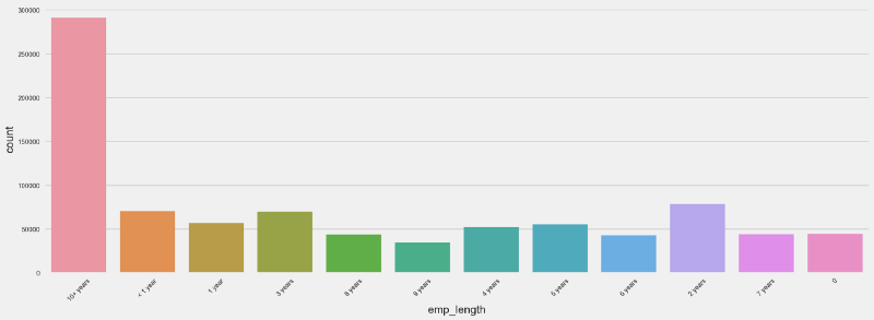Let’s see how employment length correlates with the loan status.

Since we’re talking about two categorical variables, we will generate some dummy variables and see how the pearson correlation between them looks like through a heatmap.

Unfortunately, there are no significant linear correlations between the dummy variables related to employment length and loan status.

Would the correlations between employment length and the loan grade show a different story?

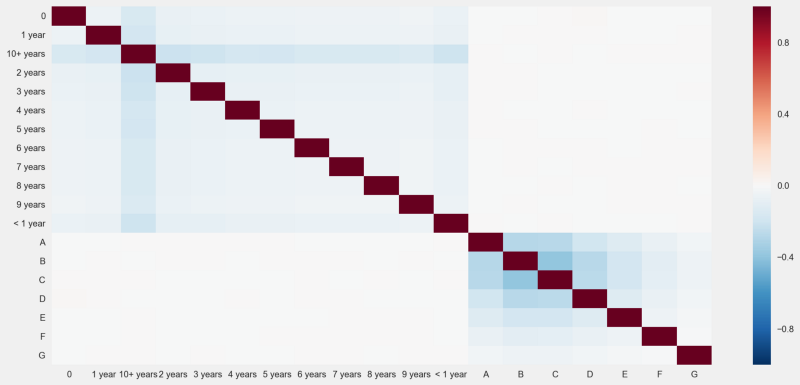Same old — no absolute correlation scores above 0.4.

Our quest does not end here, though.

We will continue expanding our analysis in a next post, where we will analyze hybrid loan x borrower characteristics, such as debt to income ratio, delinquency rates, and also other types of data such as geographic data and macroeconomic variables.

Getting to understand this public will help us achieve our objective in the longer run, which is creating a new machine learning model for predicting loan grades and credit default.

You Might Also Like

Keeping Your Machine Learning Models on the Right Track: Getting Started with MLflow, Part 2
Learn how to use MLflow Model Registry to track, register and deploy Machine Learning Models effectively.mlopshowto.comKeeping Your Machine Learning Models on the Right Track: Getting Started with MLflow, Part 1
Learn why Model Tracking and MLflow are critical for a successful machine learning projectmlopshowto.comAbout MLOps And Why Most Machine Learning Projects Fail — Part 1
If you have been involved with Machine Learning (or you are aiming to be), you might be aware that reaping the…mlopshowto.com