Deep Blue Sea: Using Deep Learning to Detect Hundreds of Different Plankton Species

In this post, we will go through a pipeline for using Keras, Deep Learning, Transfer Learning and Ensemble Learning to predict the species from hundreds of plankton species

Source: UnsplashBack in 2014, Booz Allen Hamilton and the Hartfield Marine Center at the Oregon State University organized a fantastic Data Science Kaggle Competition as part of that year’s National Data Science Bowl.

The objective of the competition was to create an algorithm for automatically classifying different plankton images as one among 121 different species. From the competition’s home page:

Traditional methods for measuring and monitoring plankton populations are time consuming and cannot scale to the granularity or scope necessary for large-scale studies. Improved approaches are needed. One such approach is through the use of an underwater imagery sensor. This towed, underwater camera system captures microscopic, high-resolution images over large study areas. The images can then be analyzed to assess species populations and distributions.

The National Data Science Bowl challenges you to build an algorithm to automate the image identification process. Scientists at the Hatfield Marine Science Center and beyond will use the algorithms you create to study marine food webs, fisheries, ocean conservation, and more. This is your chance to contribute to the health of the world’s oceans, one plankton at a time.

As part of a graduate Machine Learning course at the University of Amsterdam, students were tasked with this challenge. My team’s model finished in 3rd place among 30 other teams, with an accuracy score of 77.6% — a difference of ~0.005 between our score and the winning team.

I decided to share a bit of our strategy, our model, challenges and tools we used. We will go through the items below:

1. Deep Neural Networks: Recap
2. Convolutional Neural Networks: Recap
3. Activation Functions
4. Data at a Glance
5. Data Augmentation Techniques
6. Transfer Learning
7. Ensemble or Stacking
8. Putting it All Together

Deep Neural Networks

Source: 3Blue1BrownI will go ahead and assume that you are already familiar with the concept of Artificial Neural Networks (ANN). If that is the case, the concept of Deep Neural Networks is fairly simple. If that is not the case, this video has a great and detailed explanation about how it works. Finally, you can check out this specialization created by the great Andrew Ng if you want to gain an edge on Deep Learning.

Deep Neural Networks (DNN) are a specific group of ANNs that are characterised by having a significant amount of hidden layers, among other aspects.

The fact that DNNs have many layers allows them to perform well in classification or regression tasks involving pattern recognition problems within complex, unstructured data, such as image, video and audio recognition.

Convolutional Neural Networks

Convolutional Neural Networks (CNNs) are a specific architecture type of DNNs which add the concept of Convolutional Layers. These layers are extremely important to extract relevant features from images to perform image classification.

This is done by applying different kinds of transformations across each of the image’s RGB channels. So in layman terms, we can say that Convolution operations perform transformations over image channels in order to make it easier for a neural network to detect certain patterns.

While getting into the theoretical and mathematical details about Convolutional Layers is beyond the scope of this post, I can recommend this chapter from a landmark book on Deep Learning by Goodfellow et al to better understand not only Convolution Layers, but all aspects related to Deep Learning. For those who want to get their hands dirty, this course from deeplearning.ai is also great for getting a head start into Convolutional Neural Networks with Python and Tensorflow.

Activation Functions

Activation functions are also important in this context, and in the case of DNNs, some of the activation functions that are commonly used are ReLU, tanh, PReLU, LReLU, Softmax and others.

These functions represented a huge shift from classical ANNs, which used to rely on the Sigmoid function for activation. This type of activation function is known to suffer from the Vanishing Gradient problem; rectifying functions such as ReLU present one of the possible solutions for this issue.

Data at a Glance

Now going back to our problem. The data is composed by training and testing sets. In the training set, there are ~24K images of plankton and in the testing set there are ~6K images of plankton.

A first look at the data shows that we have an imbalanced dataset — the plot below shows how many images from each species we have in the training set.

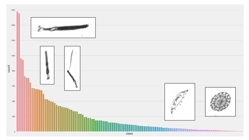Number of images in the dataset for different plankton species. Source: AuthorThis is a problem, specially for species that are under represented. Most likely our model would not have enough training data to be able to detect plankton images from these classes.

The approach we used to tackle this problem was to set class weights for imbalanced classes. Basically, if we have image classes A and B, where A is underrepresented and B is overrepresented, we could want to treat every instance of class A as 50 instances of class B.

Thismeans that in our loss function, we assign higher value to these instances. Hence, the loss becomes a weighted average, where the weight of each sample is specified by class_weight and its corresponding class.

Data Augmentation

One of the possible caveats of Deep Learning is that it usually requires huge amounts of training samples to achieve a good performance. A common approach for dealing with a small training set is augmenting it.

This can be done by generating artificial samples for one or more classes in the dataset by rotating, zooming, mirroring, blurring or shearing the original set of images.

In our case, we used the Keras Preprocessing library to perform online image augmentation — transformation was performed on a batch-by-batch basis as soon as each batch was loaded through the Keras ImageDataGenerator class.

Transfer Learning

One of the first decisions one needs to make when tackling an image recognition problem is whether to use an existing CNN architecture or creating a new one.

Our first shot at this problem involved coming up with a new CNN architecture from scratch, which we called SimpleCNN. The accuracy obtained with this architecture was modest — 60%.

With lots of researchers constantly working throughout the world in different architectures, soon we realised that it would be infeasible to come up with a new architecture that could be better than an existing one, without spending significant amounts of time and computing power training it and testing it.

With this in mind, we decided to leverage the power of Transfer Learning.

The basic idea of Transfer Learning is using existing pre-trained, established CNN architectures (and weights, if needed) for a particular prediction task.

Most deep learning platforms such as Keras and PyTorch have out of the box functionality for doing that. By using Transfer Learning, we obtained models with accuracies between 71% and 74%.

Ensemble Learning

We obtained a fairly good accuracy with Transfer Learning, but we still weren’t satisfied. So we decided to use all the models we trained at the same time.

One approach that is commonly used by most successful Kaggle teams is to train separate models and create an ensemble with the best performing ones.

This is ideal, as it allows team members to work in parallel. But the main intuition behind this idea is that predictions from an individual model could be biased; by using multiple predictions from an ensemble, we are getting a collegiate opinion, similar to a voting process for making a decision. In Ensemble Learning, we can have Hard Voting or Soft Voting.

Source: UnsplashWe opted for Hard Voting. The main difference between the two is that while in the first we perform a simple majority vote taking predicted classes into consideration, in the second we take an average of the probabilities predicted by each model for each class, selecting the most likely one in the end.

Putting it all Together

After putting all the pieces together, we obtained a model with a ~77.6% accuracy score for predicting plankton species for 121 distinct classes.

The diagram below shows not only the different architectures that were individually trained and became part of our final stack, but also a high level perspective of all the steps we conducted for our prediction pipeline.

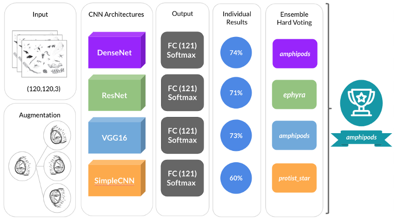A diagram showing the preprocessing, CNN architecture, training and ensembling aspects of our pipeline. Source: Author### Conclusions & Final Remarks

• Transfer Learning is excellent for optimizing time-to-market for new data products and platforms, while being really straightforward.
• Ensemble Learning was also important from an accuracy standpoint — but would probably present its own challenges in an online, real-world, production environment scenario
• As with most Data Science problems, data augmentation & feature engineering were key for getting good results

For similar problems in the future, we would try to:

• Explore a bit of offline image augmentation with libraries such as skimage and OpenCV
• Feed some basic image features such as width, height, pixel intensity and others to Keras’ Functional API

But this will be subject for a next post. In the meantime, check my other stories:

Keeping Your Machine Learning Models on the Right Track: Getting Started with MLflow, Part 2
Learn how to use MLflow Model Registry to track, register and deploy Machine Learning Models effectively.mlopshowto.comData Pipeline Orchestration on Steroids: Getting Started with Apache Airflow, Part 1
What is Apache Airflow?towardsdatascience.comData Leakage, Part I: Think You Have a Great Machine Learning Model? Think Again
Got insanely excellent metric scores for your classification or regression model? Chances are you have data leakage.towardsdatascience.com