TLDR; Github currently stores traffic metrics for only 15 days - if you want to store these metrics for a longer period you are out of luck. I wanted to have these numbers for my own repos, so in this post I will show how I have done that using Databricks, Delta, Workflows, and Databricks SQL.
Github Traffic Metrics
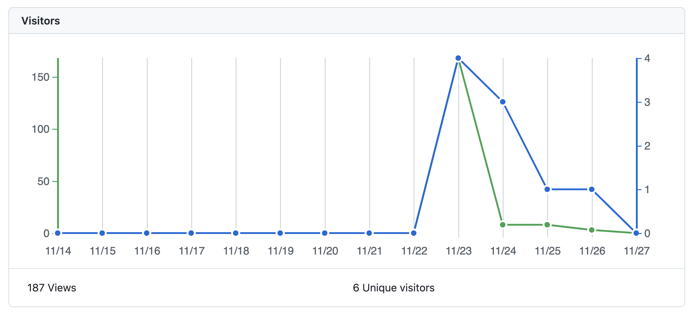
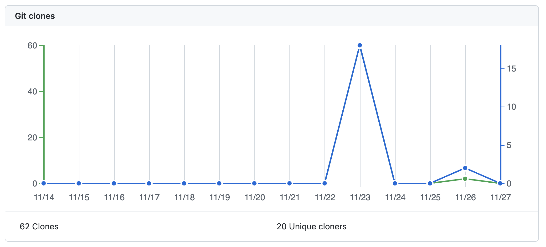
For any particular code repo, Github provides a really nice feature under the Insights tab, which indicates some analytics metrics such as number of visits and repo clones.
I have recently released Jupyter to Databricks, a simple Github Action which automatically converts all the Jupyter Notebooks from a given path in your repo to Databricks Python Notebooks. I wanted to gauge how many people were interested by it, so I looked over the metrics for the repo where I’m storing the code for this Github action (this one). This is what I found:
This is pretty neat. There’s only one issue: these are only stored for 15 days, meaning you lose everything that is older than that.
Retrieving and Storing these Metrics
Luckily, there’s a Python package that allows to easily interact with Github’s REST API: PyGithub. Most of the API endpoints are exposed in this package, and for repo statistics this is no different.
With PyGithub on my side, I just needed to schedule a process to run it and store the resulting metrics somewhere. I didn’t want to store these in a transactional database - didn’t want to bother setting up one just for the sake of this amount of data. On the other hand, if I stored this in simple cloud storage the cost would be negligible, so I thought, why not storing this in Delta?
So I coded up the following notebook to:
Authenticate with Github using a PAT Token that I generated
Iterate through all of the repos in my account and fetch traffic metrics & statistics
Store these metrics as two separate Delta tables: views and clones - I admit I was lazy to code up a MERGE statement to only insert new / non-overlapping records, but ended up just creating a separate, golden table after removing the duplicates from the raw table 😃
# Databricks notebook source
!pipinstall--upgradepip&&pipinstallpygithub# COMMAND ----------
ACCESS_TOKEN=dbutils.secrets.get(scope="github",key="github-access-token")# COMMAND ----------
fromgithubimportGithubimportosfrompyspark.sqlimportSparkSession,Rowfrompyspark.sql.typesimport(StructType,StructField,TimestampType,IntegerType,StringType)defget_repos_traffic():# using an access token
g=Github(ACCESS_TOKEN)user=g.get_user(login="rafaelvp-db")repos=user.get_repos()views_list=[]clones_list=[]forrepoinrepos:print(repo.name)views=repo.get_views_traffic(per="day")clones=repo.get_clones_traffic(per="day")list_views=[{"repo":repo.name,"uniques":view.uniques,"count":view.count,"timestamp":view.timestamp}forviewinviews["views"]]list_clones=[{"repo":repo.name,"uniques":clone.uniques,"count":clone.count,"timestamp":clone.timestamp}forcloneinclones["clones"]]views_list.extend(list_views)clones_list.extend(list_clones)schema=StructType([StructField("repo",StringType(),False),StructField("uniques",IntegerType(),False),StructField("count",IntegerType(),False),StructField("timestamp",TimestampType(),False),])spark=SparkSession.builder.getOrCreate()df_views=spark.createDataFrame(views_list,schema=schema)df_clones=spark.createDataFrame(clones_list,schema=schema)df_views.write.saveAsTable("views",mode="append")df_clones.write.saveAsTable("clones",mode="append")# COMMAND ----------
get_repos_traffic()# COMMAND ----------
spark.sql("select * from views").dropDuplicates(["repo","timestamp"]).write.saveAsTable("views_golden",mode="overwrite")spark.sql("select * from clones").dropDuplicates(["repo","timestamp"]).write.saveAsTable("clones_golden",mode="overwrite")
Orchestration
In the past, I would simply setup a VM with a cron task to run this code, or even use an existing Airflow installation and setup a DAG to run this on a schedule.
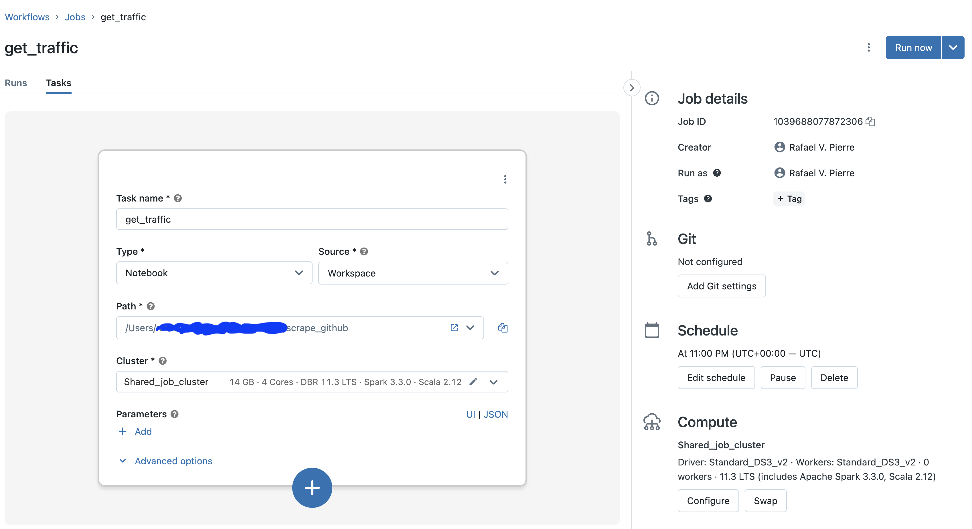
Since I wanted to simplify my life here by avoiding any kind of work related to infra setup, I went with Databricks Workflows. The workflow itself was really simple to setup, and it looks like this:
I’m using a really small, single node job cluster - this means that I’m spinning up compute with insignificant amount of cost on the fly; once the job stops running, cluster is automatically killed. 💰
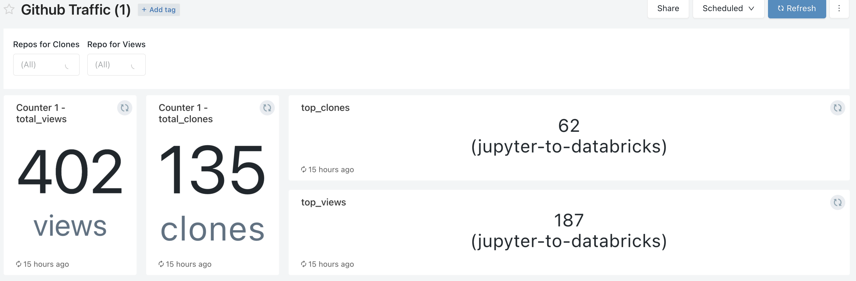
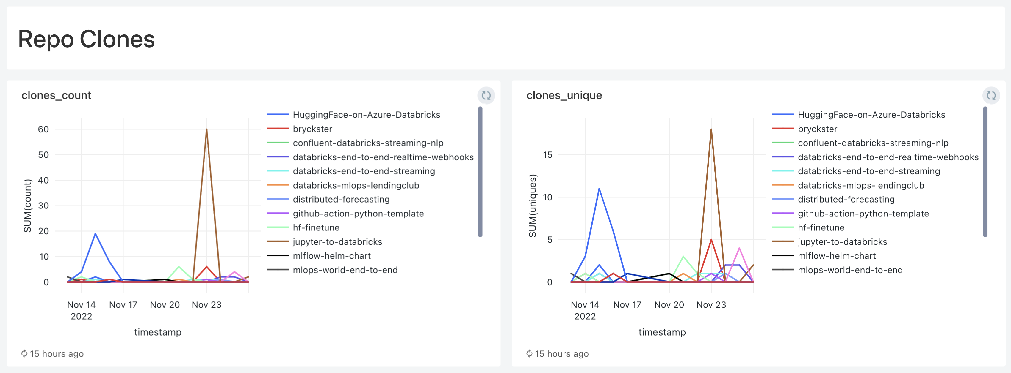
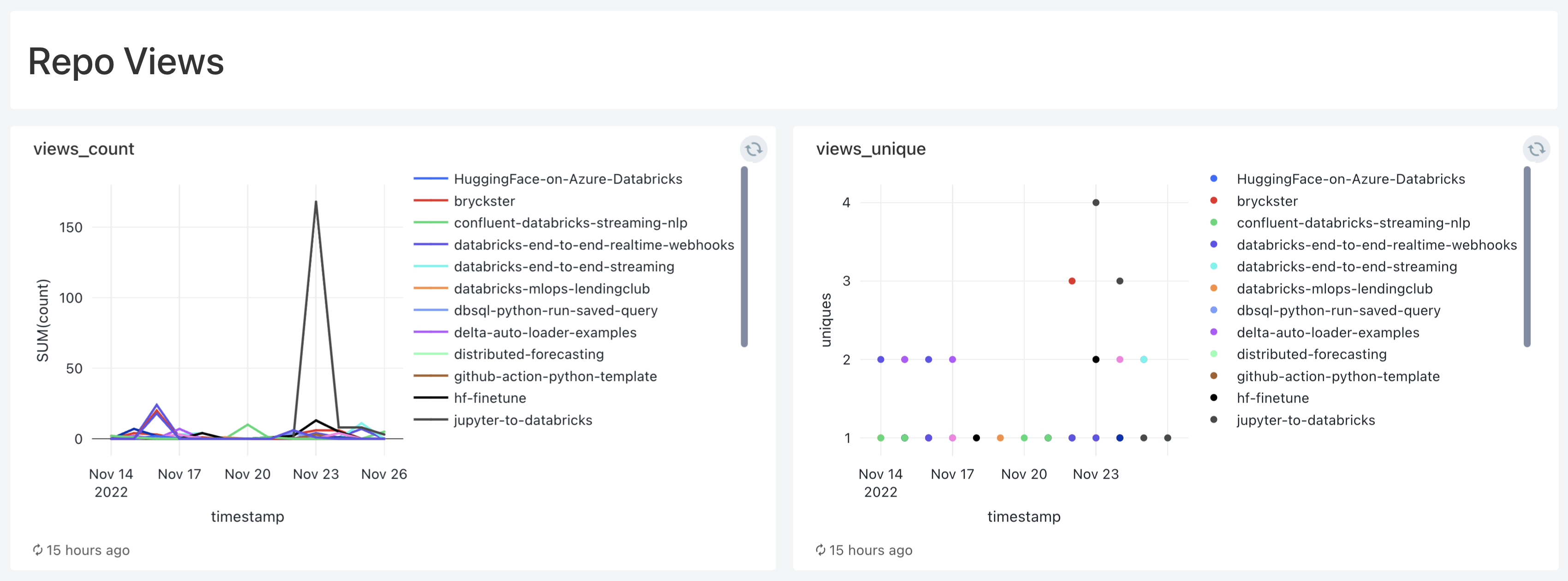
Visualization & Analytics
All right, now that I had the data, time to create some nice & insightful visualizations.
I had everything running under Databricks. So I thought, why not keep it simple and also do the analytics part with Databricks SQL?
A few queries and visualizations later, and here we are:
Takeaways
Now I can store all traffic metrics from all my repos for life 🙌🏻
TLDR; these are personal study notes on Apache Spark optimization, specially focusing on the basics but also features added after version 3.0.
Some Background on Adaptive Query Execution
Primitive version on Spark 1.6
New version prototyped and experiment by Intel Big Data
Databricks and Intel co-engineered new AQE in Spark 3.0.
Performance Optimization on Spark: Cost-Based Optimization
Prior to Apache Spark 3.0, most of the possibilities around Spark Optimization were centered around Cost-Based Optimization.
Cost-Based Optimization aims to choose the best plan, but it does not work well when:
Stale or missing statistics lead to innacurate estimates
Collecting statistics and making sure cardinality estimates are accurate is costly, so this is something users struggled with. It could also be that your data hasn’t changed; in this case you would be doing unecessary recalculations.
Statistics collection are too costly (e.g. column histograms)
Predicates contain UDFs
Hints do not work for rapidly evolving data
Adaptive Query Execution, on the other hand, bases all optimization decisions on accurate runtime statistics.
Query Stages
Shuffle or broadcast exchanges divide a query into query stages
Intermediate results are materialized at the end of a query stage
Query stage boundaries optimal for runtime optimization:
The inherent break point of operator pipelines
Statistics available, e.g. data size, partition sizes
TLDR; MLflow Model Registryallows you to keep track of different Machine Learning models and their versions, as well as tracking their changes, stages and artifacts.Companion Github Repofor this post
In our last post, we discussed the importance of tracking Machine Learning experiments, metrics and parameters. We also showed how easy it is to get started in these topics by leveraging the power of MLflow (for those who are not aware, MLflow is currently the de-facto standard platform for machine learning experiment and model management).
In particular, Databricks makes it even easier to leverage MLflow, since it provides you with a completely managed version of the platform.
This means you don’t need to worry about the underlying infrastructure to run MLflow, and it is completely integrated with other Machine Learning features from Databricks Workspaces, such as Feature Store, AutoML and many others.
Coming back to our experiment and model management discussion, although we covered the experiment part in the last post, we still haven’t discussed how to manage the models that we obtain as part of running our experiments. This is where MLflow Model Registry comes in.
The Case for Model Registry
As the processes to create, manage and deploy machine learning models evolve, organizations need to have a central platform that allows different personas such as data scientists and machine learning engineers to collaborate, share code, artifacts and control the stages of machine learning models. Breaking this down in terms of functional requirements, we are talking about the following desired capabilities:
discovering models, visualizing experiment runs and the code associated with models
transitioning models across different deployment stages, such as Staging, Production and Archived
deploying different versions of a registered model in different stages, offering Machine Learning engineers and MLOps engineers the ability to deploy and conduct testing of different model versions (for instance, A/B testing, Multi-Armed Bandits etc)
archiving older models for traceability and compliance purposes
enriching model metadata with textual descriptions and tags
managing authorization and governance for model transitions and modifications with access control lists (ACLs)
Now to the practical part. We will run some code to train a model and showcase MLflow Model Registry capabilities. Hereby we present two possible options for running the notebooks from this quickstarter: you can choose to run them on Jupyter Notebooks with a local MLflow instance, or in a Databricks workspace.
Jupyter Notebooks
If you want to run these examples using Jupyter Notebooks, please follow these steps:
Run the first notebook jupyter/01_train_model.ipynb. This will create an experiment and multiple runs with different hyperparameters for a diabetes prediction model.
Run the second notebook jupyter/02_register_model.ipynb. By doing so, we will register our model artifact into MLflow model registry. We will also do some basic sanity checks in order to confirm that our model can be promoted to Staging.
For this example we are running a simple, local instance of MLflow with a SQLite backend — which is good enough for a toy example, but not recommended for a test or production setup. It is also possible to run MLflowlocally or remotely as a standalone web application, and also with a Postgresql backend. For more details on how to achieve this, please refer to the different scenarios presented in this link.
Run the first notebook databricks/01_train_model.py.
Run the second notebook databricks/02_register_model.py.
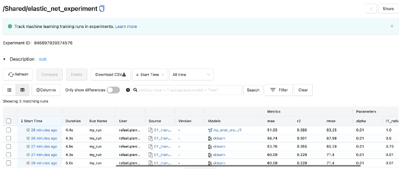
Bonus 1: if you run these notebooks on a Databricks Workspace, you will be able to visualize the different runs associated with your experiment:
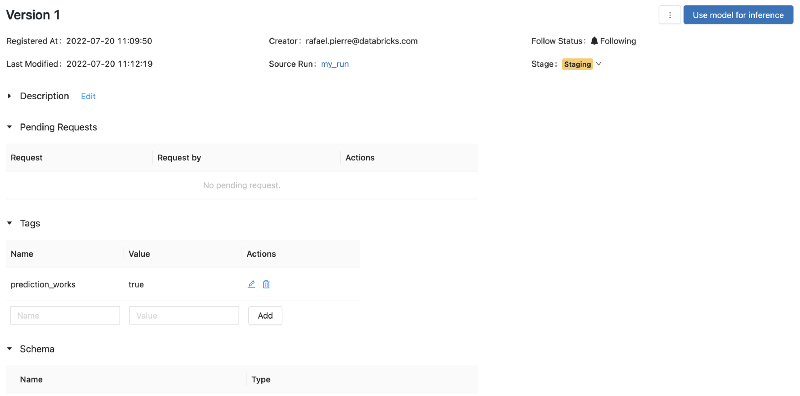
Looking at the screenshot above, you might notice that on the first row of our table, in the models column, we have an icon which differs from the other rows. This is due to the fact that the model artifact for that specific run was registered as a model, and a new model version was created (version 1). If we click on its link, we get redirected to the following window.
In the window above, we have an overview of the model version that was registered. We can see that it has the tag prediction_works = true. We can also see that it is in Staging. Depending on which persona is accessing this data, it might be possible to manually change the stage (to promote the model to Production, for instance), or reverting it back to None.
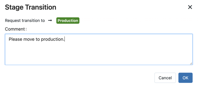
Moreover, with Workspace Object Access Control Lists, you could limit the permissions for each type of user. Let’s say that you wish to block data scientists from transitioning model stages, while you want to allow team manager to do so. In such scenario, Data Scientists would have to request transitions to a given stage.
These transitions would then need to be approved by someone with the right permissions. Finally, all of the requests and model stage transitions are tracked in the same window (and of course, they are also available programatically).
Once a model has been transitioned to Production, it is quite simple to deploy it either as an automated job or as a Real time REST API Endpoint. But that is the topic for another post.
All the code used in this post is available on the Github repo below:
UPDATE (28/05/2022): *Podman covers most of Docker functionality, however I found that image layer caching is currently missing. One solution is using Podman coupled with buildkit.
While it is possible to request a license for it, a great open source alternative is to use Podman.
TLDR from their website: “Podman is a daemonless container engine for developing, managing, and running OCI Containers on your Linux System. Containers can either be run as root or in rootless mode. Simply put:alias docker=podman. More detailshere.”
How to install it and run it
On a macOS it’s pretty easy:
brew install podman
Once it’s installed, you need to create a virtual machine. This can be done by running:
podman machine init
This should have created a virtual machine which will be used as our backend for everything Podman related. Let’s go on and start our virtual machine with:
podman machine start
Our virtual machine should be running & ready to use. We can double check by running:
podman machine list
Usage
The Podman CLI uses the same conventions and parameters as Docker’s, which is pretty neat. You can even create an alias for it, so that you can fire it up using the good and old docker command. Just add the following to your .bash_profile (or.zshrc, if you use ZShell):
alias docker=podman
And you’re done. You can test it quite easily by pulling an image:
docker pull busybox
Troubleshooting
Unable to start host networking
It could be that you come across this error when trying to start Podman’s VM (podman machine start):
Error: unable to start host networking: “could not find \”gvproxy\” in one of [/usr/local/opt/podman/libexec /opt/homebrew/bin /opt/homebrew/opt/podman/libexec 3/usr/local/bin /usr/local/libexec/podman /usr/local/lib/podman /usr/libexec/podman 4/usr/lib/podman]”
To solve that, from a terminal window run:
vim ~/.config/containers/containers.conf
In the engine section, add the following line (replace 4.1.0 with your version if needed):
Your final containers.conf file should look like this:
QEMU
QEMU is a virtualization engine for Mac. Depending on your environment, you might also need to install it. Easy to do it with brew:
brew install qemu
Now you should be good to go 😄
Podman Compose
You might be asking: what about Docker Compose? Well, I’ve got some good news for you: there’s Podman Compose!
To install it:
pip3 install podman-compose
You can run it in the same way as Docker Compose. From a directory containing your docker-compose.yaml, simply run:
podman-compose up
Needless to say — you could also create an alias for it:
alias docker-compose=podman-compose
Bonus: Using Podman to Migrate from Docker Compose to Kubernetes
One challenge with Docker Compose is that the YAML file format only works with the Docker engine. While you can give it to other Docker users for local replication, they cannot use it with other container runtimes. That is, until now.
There’s a nice bonus with Podman: you can use it to convert package the containers that you have previously spun up with Docker Compose to Kubernetes YAML Manifests.
You cannot understand what is happening today without understanding what came before (Steve Jobs)
Machine Learning as an Empirical Science — and the importance of experiment tracking
Empirical research is an evidence-based approach to the study and interpretation of information. The empirical approach relies on real-world data, metrics and results rather than theories and concepts. Empiricism is the idea that knowledge is primarily received through experience and attained through the five senses.
In order to validate our initial hypothesis, we work with the assumption that our experiments are sufficiently robust and successful. As a byproduct, we would end up with a model which is able to predict outcomes for previously unseen events, based on the data which was used for training.
Of course, reality is much more nuanced, complex — and less linear— than that. More often than not we will need to test many different hypothesis, until we find one that while not bad, is mediocre at best. Many iterations later, we might end up with a satisfactory model.
The case for Machine Learning Model Tracking
Being able to look back into different machine learning experiments, their inputs, parameters and outcomes is critical in order to iteratively improve our models and increase our chances of success.
One reason for this is that the cutting edge model that you spent days training last week might be no longer good enough today. In order to detect and conclude that, information about the inputs, metrics and the code related to that model must be available somewhere.
This is where many people might say — I’m already tracking this. And my hundred Jupyter Notebooks can prove that. Others might say something similar, while replacing Jupyter Notebooks with Excel Spreadsheets.
How a folder full of different Jupyter Notebooks looks likeWhile none of these approaches is inherently wrong, the process gets challenging and error-prone once you start to move along three scales:
Number of use cases and models;
Scale of your team;
Variety of your models (and data)
In other words, you do not want to rely on Jupyter Notebooks and Excel spreadsheets when you are running production grade machine learning systems — you need something structured and flexible, which enables seamless collaboration amongst different people and personas.
Introducing MLflow
MLflow is an open source project that was created by Databricks — the same company behind Apache Spark and Delta, amazing open source projects as well.
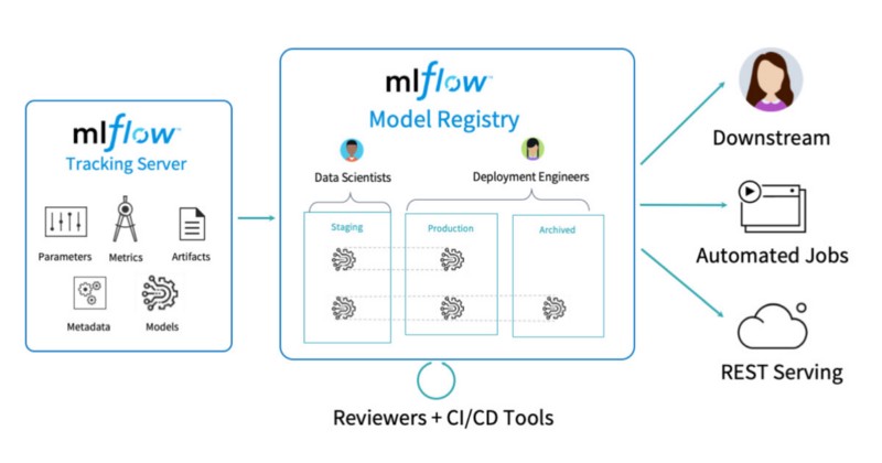
The main objective of MLflow is to provide a unified platform for enabling collaboration across different teams involved in creating and deploying machine learning systems, such as data scientists, data engineers and machine learning engineers.
A typical Machine Learning workflow using MLflowIn terms of functionalities, MLflow allows tracking Machine Learning experiments in a seamless way, while also providing a single source of truth for model artifacts. It has native support for a wide variety of model flavors— think plain vanilla Sci-Kit Learn, but also models trained with R, SparkML, Tensorflow, Pytorch, amongst others.
Getting Started
Now that we know about experiment tracking, MLflow and why these are important in a Machine Learning project, let’s get started and see how it works in practice. We will:
Create a free Databricks Workspace using Databricks Community Edition
Create multiple runs for a machine learning experiment
Compare these experiment runs
Look at the artifacts that were generated by these runs
Databricks Community Edition
The first step is signing up to Databricks Community Edition, a free version of the Databricks cloud based big data platform. It also comes with a rich portfolio of award-winning training resources that will be expanded over time, making it ideal for developers, data scientists, data engineers and other IT professionals to learn Apache Spark. On top of that, a managed installation of MLflow is also included.
Simply click on this link to get started. Once you register and login, you will be presented with your Databricks Workspace.
2. Creating a compute cluster
In your workspace, you are able to create a small scale cluster for testing purposes. To do so, on the left hand side menu, click on the Compute button, and then on the Create Cluster button.
It is recommended to choose a runtime that supports ML applications natively — such runtime names end with LTS ML. By doing so, MLflow and other common machine learning frameworks will automatically be installed for you. Choose a name for your cluster and click create.
3. Importing our Experiment Notebook
Next, you will want to create a Databricks Notebook for training your model and tracking your experiments. To make things easier, you can import an existing quickstart notebook — but of course, if you prefer to write your own code to train your model, feel free to do so. The MLflow Quickstart Notebook used for this exercise can be found here.
In a nutshell, our quickstart notebook contains code to train a Machine Learning model to predict diabetes using a sample dataset from Sci-Kit Learn. The notebook is really well documented and contains all the details about the model and the different training steps.
How to import an existing Databricks Notebook4. Running Your Notebook and Training Your Model
The next step is running your notebook and training your model. To do so, first attach the notebook to the cluster you have previously created, and click the Run All button.
If you are using our quickstart notebook, you will notice that each time you train your model with different parameters, a new experiment run will be logged on MLflow.
To have a quick glance on how each experiment run looks like, you can click on the experiments button at the top right of your notebook.
A more detailed view on your experiments is available on the Machine Learning UI.
How to access the Databricks Machine Learning UIOnce you are on the Machine Learning UI, you can click on the Experiments button on the bottom of the left hand side menu. Doing so will display a detailed view of your different model runs.
5. Comparing and Analysing Experiment Runs
You can visually compare hyperparameters and metrics of different experiment runs. To do so, select the models you want to compare by clicking on their checkboxes on the left hand side of the main table, and click Compare.
By doing so, you will be able to inspect different hyperparameters that were used across experiment runs, and how they affect your model metrics. This is quite useful to understand how these parameters influence your model performance and conclude which set of parameters might be best — for deploying the final version of your model into production, or for continuing further experiments.
The great thing is that these results are available for you, but in a team setting, you could also share these with a wider team of Data Scientists, Data Engineers and Machine Learning Engineers.
6. Model Artifacts
In our quickstart notebook, we have code for logging model parameters (mlflow.log_param), metrics (mlflow.log_metric) and models (mlflow.sklearn.log_model).
When you select a particular model from the table containing all experiment runs, you can see additional information related to that model, and also the artifacts related to that model.
This is also quite useful for when you want to deploy this model into production, since amongst the artifacts, you will have not only the serialized version of your model, but also a requirements.txt file containing a full list of Python environment dependencies for it.
### Main Takeaways
By this point you should have understood:
Why Machine Learning Experiment Tracking is critical for success when running production grade ML
How MLflow makes it seamless to track Machine Learning experiments and centralize different model artifacts, enabling easy collaboration in ML teams
How easy it is to train your models with Databricks and keep them on the right track with MLflow
There are some more important aspects to be covered, specially when we talk about model productionization and MLOps. But these will be the topic of a next post.


 TLDR from their website: “Podman is a daemonless container engine for developing, managing, and running OCI Containers on your Linux System. Containers can either be run as root or in rootless mode. Simply put: alias docker=podman. More details
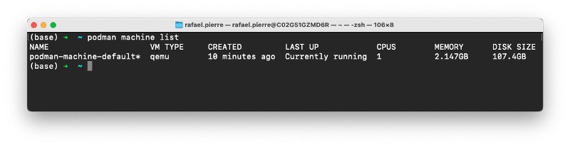
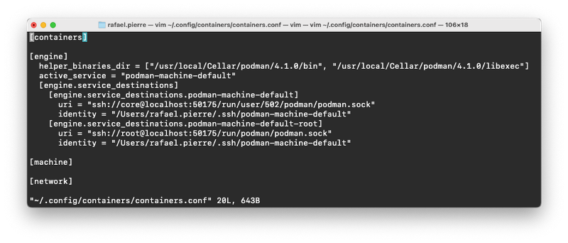
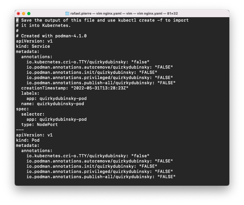
 Photo by
  E
E How a folder full of different Jupyter Notebooks looks likeWhile none of these approaches is inherently wrong, the process gets challenging and error-prone once you start to move along three scales:
 MLflow is an open source project that was created by
 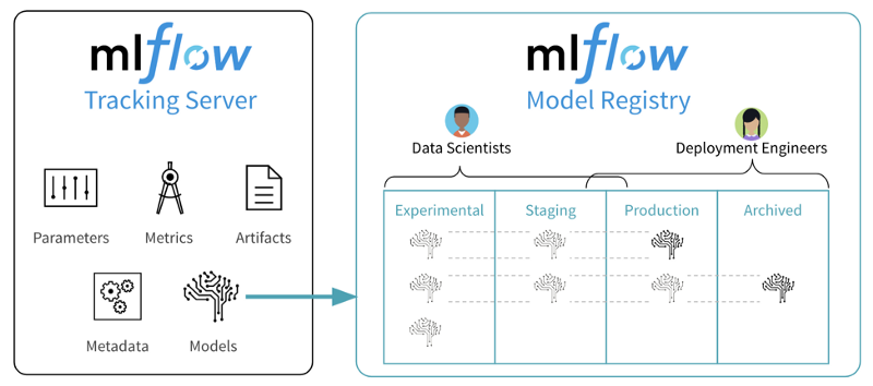 A typical Machine Learning workflow using MLflowIn terms of functionalities, MLflow allows tracking Machine Learning experiments in a seamless way, while also providing a single source of truth for model artifacts. It has native support for a wide variety of model flavors— think plain vanilla Sci-Kit Learn, but also models trained with R, SparkML, Tensorflow, Pytorch, amongst others.
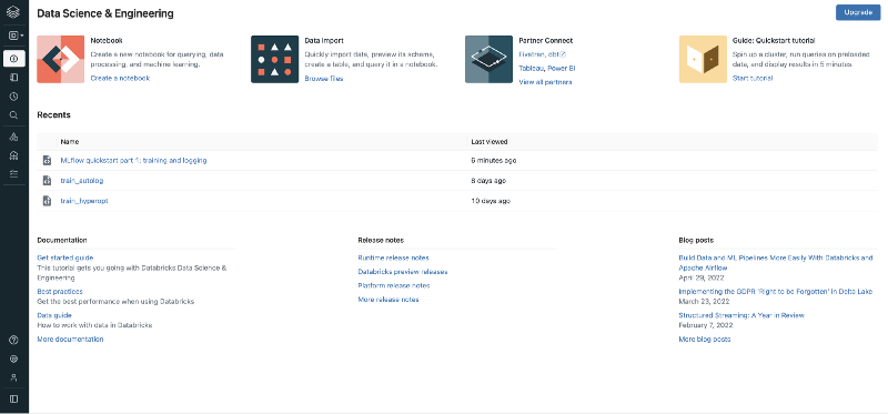 2. Creating a compute cluster
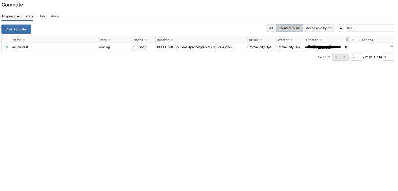 3. Importing our Experiment Notebook
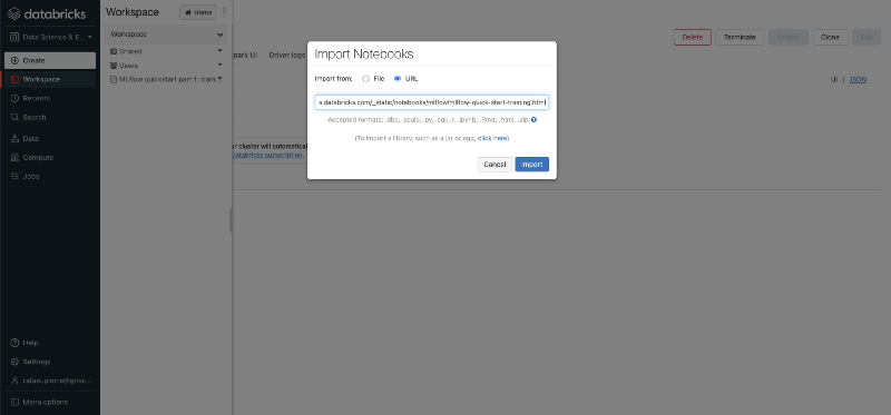 How to import an existing Databricks Notebook4. Running Your Notebook and Training Your Model
 How to access the Databricks Machine Learning UIOnce you are on the Machine Learning UI, you can click on the Experiments button on the bottom of the left hand side menu. Doing so will display a detailed view of your different model runs.
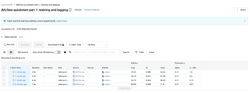 5. Comparing and Analysing Experiment Runs
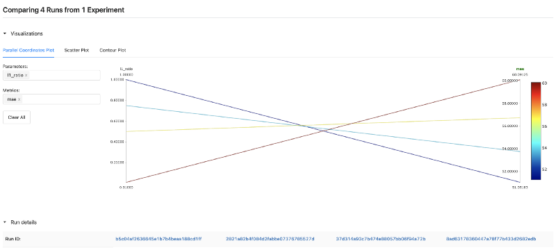 The great thing is that these results are available for you, but in a team setting, you could also share these with a wider team of Data Scientists, Data Engineers and Machine Learning Engineers.
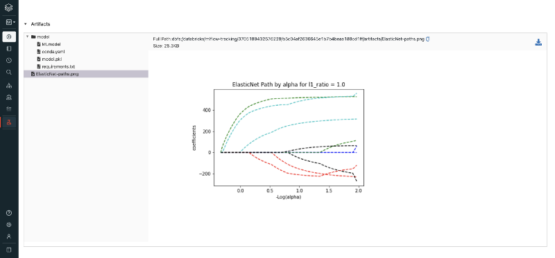 ### Main Takeaways